Preface

Over the past couple of months, I’ve been working on my rendering engine. I’ve added a couple of interesting features, and so this post goes in detail about them. 1

Skyboxes

A technique that has always bamboozled 10 year old me was skyboxes. How was my potato of a machine able to render entire worlds in its vastness? Turns out they didn’t.

A cheap yet very effective technique is to add cubemaps as skyboxes. Cubemaps are but glorified cubes (which in turn are 6 textures bound together!), with one neat trick. To sample from a cubemap, all you need is a 3-dimensional vector! An intuitive understanding of how to sample from a cubemap would be to think of standing inside the cube, right at the center, then based off the 3 vector coordinates, you pick what color to display.

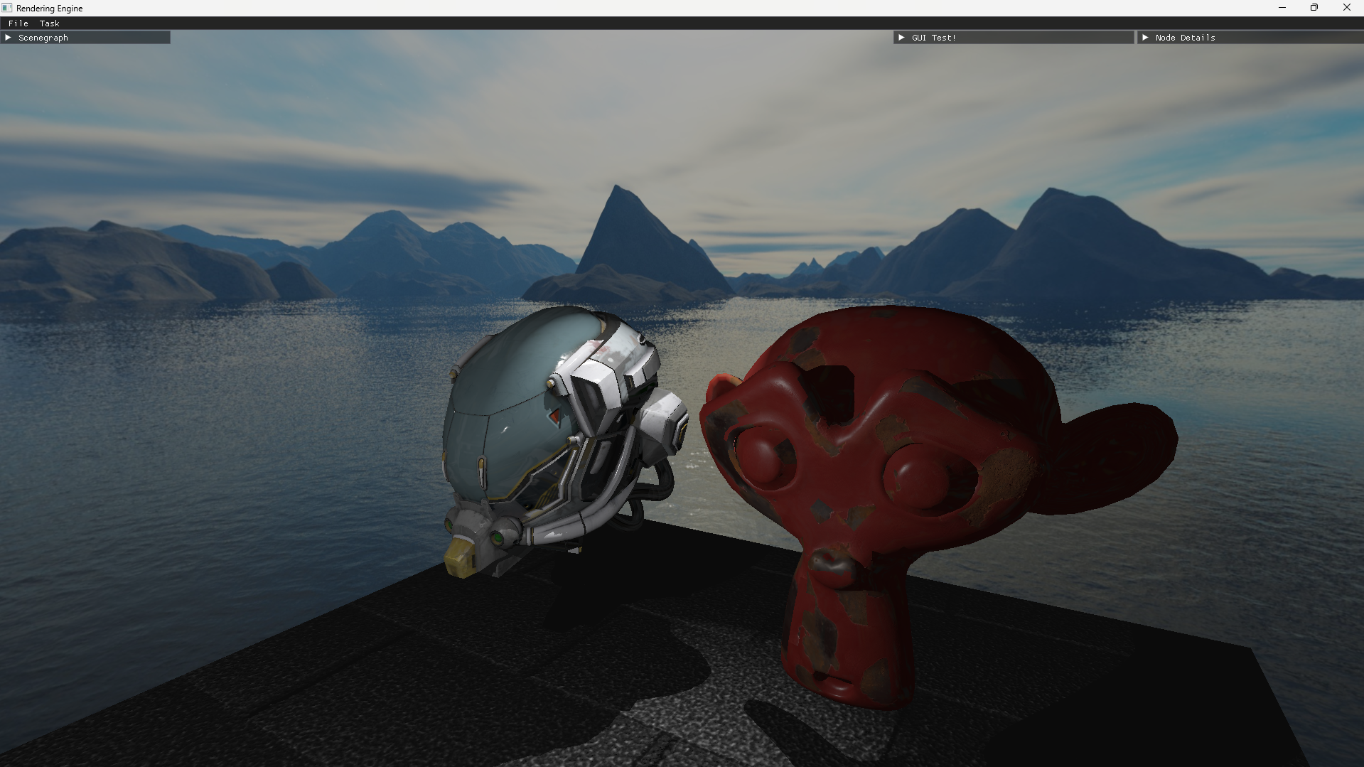
A really neat effect is that if the cube is excluded from the modelview transformation, it gives the effect of being far away from the player, which adds a bit to the realism. I’ve added cubemaps to our scene, and this is the effect:

IBL

Now that we’ve added cubemaps, it would be amazing to use them as a backdrop while rendering! Lucky for us, some very smart people have already done so, and I’ve managed to create a satisfactory replication of the same. This technique is called IBL. 2

IBL stands for Image Based Lighting, which is usually split into two parts:

• Diffuse irradiance
• Specular IBL

Diffuse

This is pretty straightforward. The diffuse part of the rendering equation is as follows:

Now, if you look closely, we see that this does not depend on the viewing direction, and we have every required variable before rendering the scene. This gives us the opportunity to pre-calculate this expensive computation and save it somewhere, and use it later when rendering in realtime! We do this through a technique called covolution, which is basically a way to compute the value in a dataset considering all the other values in the same dataset.

We will save this result in yet-another cubemap called an “environment-map”, and we will do so by discretely sampling a large number of directions \(w_i\) over the hemisphere $Ω$ and averaging their radiance. I don’t want to bore over the (albeit incredible) details, but anyone interested can read this link. 3

Specular

Now this is a bit tricky, because the specular component requires the viewing direction, which we would not have beforehand to precompute. (Besides, if we move around, we’d essentially have to recompute again). 4

To solve this problem, we have the “Split-sum approximation”. This basically says that:

can be split into:

While this is not mathematically accurate, it provides us a close enough approximation, and most importantly, it provides us a way, with some reasonable approximations, to precalculate even the specular components!

The first part is called the pre-filtered environment map. Here, we make the assumption that the view direction is equal to the normal/sampling direction, and thus equal to the reflection direction as well. With the reflection details now available and the ability to store rougher details in the higher mips of the texture, we can build the pre-filter map.

Monte-carlo?

Now to get an intuitive understanding of the specular pre-computation, I like to think of it this way: We already have the view direction, and we have the surface normals from the PBR reflectance equation. So we can work our way backwards, and find the exact light samples in the cubemap that will contribute to the specular lighting at this viewing direction.

Monte-carlo integration is a very powerful tool because it provides us a way to approximate the value of a continuous integral using discrete samples. If the samples are randomly drawn, we can eventually get a very accurate result, but they will take a lot of time to converge. On the other hand, we can choose to use a biased sample generator, so that we will converge to the result faster, but then, by nature of it being biased, we will never get a perfectly accurate result. This is completely fine for our use case, and we will generate sample vectors biased towards the general reflection orientation. This method is called “Importance Sampling”.

BRDF

The second part of the split sum approximation deals with only 2 variables, the roughness and the angle between \(n_0\) and \(omega_0\). Surprisingly, this is independent of the scene itself, and can be precalculated, and stored in a 2D LUT (look-up texture).

Too much text?

With all the context above, we have the following beauty:

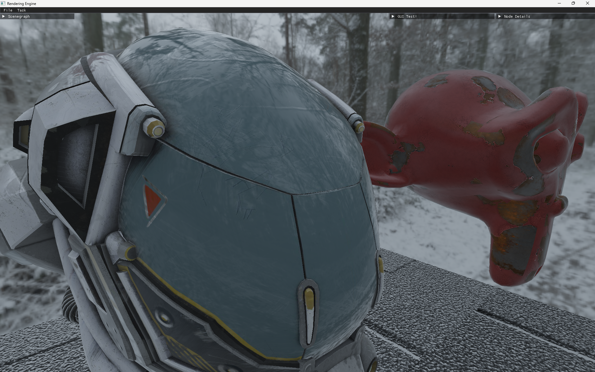
Note how the reflection on the helmet looks! It’s reflecting the branches from the skybox!

Global Illumination

Now this is a topic that is worth a post of it’s own, but I’m also lazy, so here goes nothing:

Global Illumination is a group of techniques that focus on the indirect illumination of a pixel. Now global Illumination (or GI when short) is a costly affair. You’d need to ray-trace the entire scene multiple times each frame, to get the indirect illumination at a point. There are multiple ways of achieving this, and one of them is called VXGI, which is what we will be using.

VXGI (from my admittedly novice experience) can be split into two parts : Diffuse and Specular (Once again!!!)

the basic idea is to (once again!) abuse the mip-mapping of a 3d Texture to cast cones instead of rays into the scene. This way, we’d have to sample much lesser, and we’d get a very good approximation.

The entire process is split into 3 parts:

• Voxelize the scene, and save the lighting data in a 3D texture
• Mipmap the 3D texture, so that we can sample lesser.
• use the mipmapped 3d texture to raymarch in the scene, get occlusion details, indirect diffuse and indirect specular components.

Voxelization

The idea is fairly straightforward, voxelize every polygon in your scene, and save the lighting data of each voxel in a 3D image. We use a geometry shader, and in my specific implementation, I’m using a Nvidia specific extension (there are alternatives for other GPUs). We swizzle every polygon to face the screen, and use the world-data to encode the lighting data into a 3D texture. Note that we have to use ImageAtomics here, because if there are multiple polygons that map to the same voxel, the one with the highest light intensity must be saved. The shaders for this process can be found here. 5

A Voxelized scene is shown above. Note how the scene looks much blockier!

Mipmaps

Usually, we’d be able to use glGenerateMipmaps() and call it a day, but not when it happens every frame. The implementation of that method is pretty poor, and I had to use a compute shader to manually generate the mipmaps of the 3d texture. The compute shader code can be found here. 6

Raymarching

The stage has been set, we can finally raymarch through the scene and get our required indirect illumination data! We do this by setting up some widely oriented cone directions, then for each fragment we’d have to shoot rays in these cone directions, but instead of shooting multiple rays, we’d sample the higher mips. This gives us a good way of taking multiple samples without necessarily shooting multiple rays. (Genius, right?!)

So we raymarch with cones 3 times:

• Once to find any objects that might be occluding the current fragment from light. This produces us soft shadows.
• Once to find the diffuse component of indirect lighting. This will draw lighting data by raymarching multiple cones.
• Once to find the specular component of indirect lighting. This will use a singular, much narrower cone that is oriented based off the view vector.

couple of points worth mentioning:

• a depth pre-pass is absolutely necessary. This is because the final fragment shader is very heavy, so we really want to do it only once for every fragment that shows up on the screen.
• the occlusion check is done once for each light, but the specular and diffuse components are done only once for each fragment. This will very likely benefit from deferred rendering/clustered rendering.

The source code of the final pass can be found here. 7

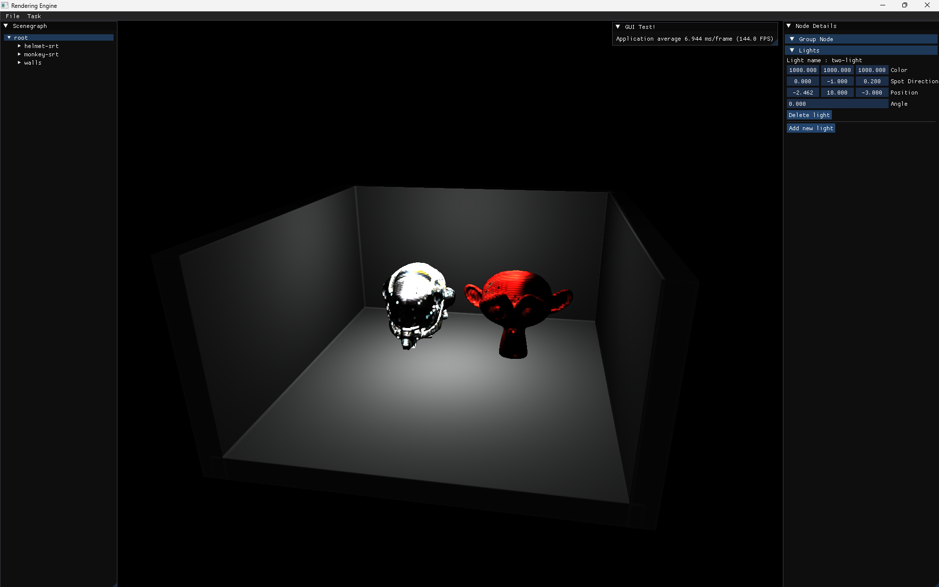
Now, for the final preview:

The first couple of seconds are with GI off, and then with GI on. Note the difference!

If you are interested in browsing through the code on the CPU side, here is a good starting point. 8

What’s next?

Well I’ve gone through some advanced(I’d like to think, atleast!) OpenGL concepts. I’ve learnt some really good Modern OpenGL, not just from implementing, but also from reading other people’s code.

For now, I’m moving on to Vulkan, and once again, I’ll be stepping into Global Illummination, except with some new specialized techniques like RTGI with ReSTIR and so on.

I hope you’ve had an interesting read. Thanks for stopping by!

References and Acknowledgements

My very thanks to prof. Amit Shesh, without whom this project would have never reached the state it is in right now.

• Wicked Engine’s blog post on global illumination 9
• IDKEngine’s GI Illumination 10
• NVIDIA’s original VXGI paper 11

and many more references, I will update this once I remember any!